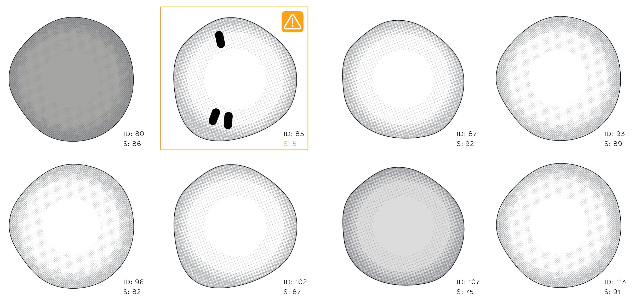
Medical images are often discussed as if they presented one problem: feed pixels into a neural network and predict a diagnosis. In practice, the more interesting work starts earlier. What is the unit of analysis—a tissue patch, an individual cell, or a parasite stage? How should rare classes be handled? Which errors matter most? And how can several model families be compared without turning an experimental notebook into an unreliable collection of disconnected cells?
I did a small excercice to explore those questions across two related computer-vision tasks:
- detecting tumour tissue in histopathology patches from the PatchCamelyon workflow;
- identifying malaria-infected blood cells, then extending the task to six cell and parasite classes.
The project was not intended as a clinical product. It was a hands-on study of the engineering and evaluation choices that make pathology models useful, reproducible, and interpretable.
One workflow, three levels of model complexity
The first part of this project compares three approaches to binary tumour-patch classification.
1. A small CNN built from scratch
The baseline is deliberately simple: three convolutional blocks followed by a compact classifier. A model like this is fast to train and easy to inspect. More importantly, it creates a reference point. Without a credible baseline, it is difficult to know whether a larger pretrained network is actually adding value.
This experiment also makes augmentation easy to test in isolation. Horizontal and vertical flips, together with mild brightness and contrast variation, encode transformations that are plausible for histology patches while leaving validation images untouched.
2. ResNet18 with transfer learning
The second model adapts an ImageNet-pretrained ResNet18. This tests whether generic visual features—edges, textures, shapes, and spatial patterns—transfer to pathology.
I organized the notebook to support both a quick full-network fine-tune and a two-stage strategy: train the new classification head first, then unfreeze the backbone with a lower learning rate. The latter is more controlled when the target dataset is smaller or visually different from the pretraining domain.
3. Phikon-v2 as a pathology foundation model
The third approach uses a frozen pathology-specific backbone to extract feature vectors, then trains lightweight linear and multilayer-perceptron heads on those cached features. This separates representation learning from downstream classification and makes repeated head experiments much cheaper.
The recorded comparison suggested the expected progression: approximately 0.93 ROC AUC for the small CNN and ResNet experiments, and approximately 0.97 ROC AUC for the Phikon-based approach. These are experiment records from the original PCam work; after reorganizing the notebook, I syntax-validated every code cell but did not rerun the full pipeline because the large HDF5 data and model download were not available in that final environment.
That distinction matters. A clean notebook is not evidence that an experiment has been reproduced. The article should say which results were rerun and which were retained from earlier runs.
Turning an experimental notebook into a reliable comparison
The original notebook contained useful experiments, but shared state made them fragile. Imports and dataset code were duplicated. Data loaders were stored in global variables and later reused for a different model. Eventually, a CNN received cached feature vectors intended for the foundation-model head, producing a shape mismatch.
The fix was architectural rather than cosmetic:
- define the dataset, training loop, evaluation, prediction, and plotting utilities once;
- pass data loaders explicitly into training functions;
- give each model its own clearly named loaders;
- apply the same evaluation sequence to every model;
- separate optional, expensive experiments from the default path.
This made the notebook read like an experiment rather than a transcript: shared setup, Model A, Model B, Model C, then a comparison. It also removed a class of hidden-state bugs common in long-running notebooks.
Moving from tissue patches to individual cells
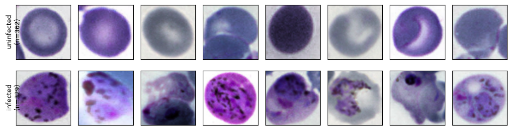
The malaria dataset changed the scale of the problem. Instead of classifying a fixed tissue tile, the pipeline reads image annotations, extracts crops around individual cells, resizes them to 64 × 64 pixels, and caches the resulting arrays for repeatable training.
The first task was binary: infected versus uninfected.
The small CNN reached 95.08% validation accuracy and 0.9872 ROC AUC on 691 held-out cell crops. Its confusion matrix contained 18 missed infected cells and 16 false alarms at the default 0.5 threshold.
Transfer learning produced a substantial improvement. ResNet18 reached 98.55% validation accuracy and 0.9977 ROC AUC, with 4 missed infected cells and 6 false alarms at the same threshold.
| Binary malaria model | Validation accuracy | ROC AUC | False negatives | False positives |
|---|---|---|---|---|
| Small CNN | 95.08% | 0.9872 | 18 | 16 |
| ResNet18 | 98.55% | 0.9977 | 4 | 6 |
These numbers illustrate why accuracy alone is insufficient. In a screening context, a false negative is not interchangeable with a false positive. Missing an infected cell and asking a reviewer to inspect an extra candidate carry different consequences.
The threshold is part of the model
A binary classifier outputs a score, not a clinical decision. The familiar threshold of 0.5 is only a default.
For the small CNN, lowering the threshold from 0.5 to 0.25 increased infected-cell recall from 94.5% to 98.2%. Missed infected cells fell from 18 to 6, while false alarms rose from 16 to 46. The threshold sweep makes that trade-off visible instead of hiding it behind a single accuracy value.
The ROC curve summarizes ranking performance over all thresholds. An AUC of 0.9977 means the ResNet scores a randomly selected infected cell above a randomly selected uninfected cell roughly 99.77% of the time. It does not, by itself, select the operating point. That choice still depends on the intended workflow and the relative cost of each error.
Beyond infected or uninfected
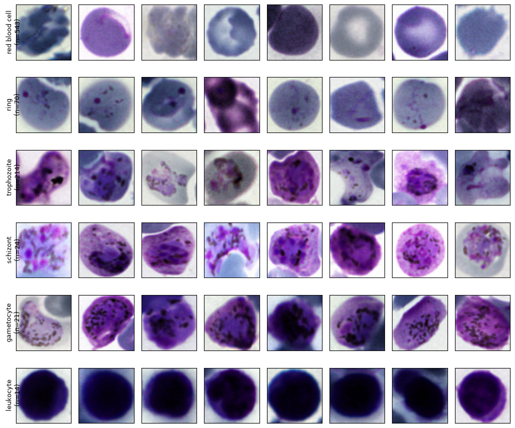
Binary classification is useful for screening, but it discards biological detail. The next model classified six categories:
- red blood cell;
- ring;
- trophozoite;
- schizont;
- gametocyte;
- leukocyte.
The annotations were extremely imbalanced: 77,420 red blood cells, compared with 1,473 trophozoites, 353 rings, 179 schizonts, 144 gametocytes, and 103 leukocytes. A further 441 objects were labelled “difficult”; I excluded that ambiguous category from supervised training.
Simply optimizing raw accuracy would encourage the model to favor the dominant red-blood-cell class. I therefore capped the number of red blood cells sampled per image, used a class-weighted cross-entropy loss, split the data by source image rather than by crop, and selected the best checkpoint using balanced accuracy.
The executed six-class ResNet achieved:
- 90.74% overall accuracy;
- 84.04% balanced accuracy in the final epoch;
- a best validation balanced accuracy of 84.88% during training;
- 0.98 F1 for red blood cells and 0.97 F1 for leukocytes;
- 0.76 F1 for rings and 0.87 F1 for trophozoites;
- 0.55 F1 for both schizonts and gametocytes.
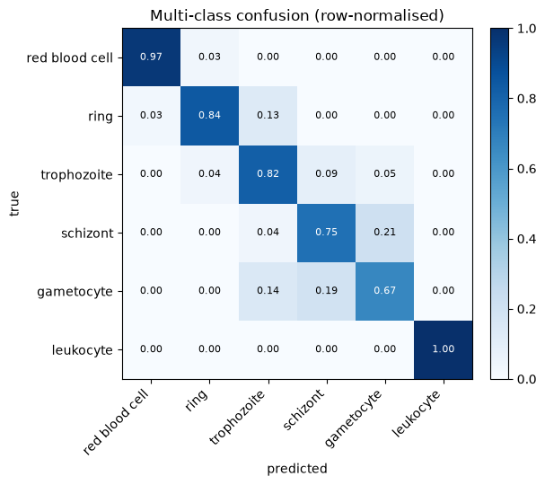
The confusion matrix exposed the main limitation: rare parasite stages were harder to distinguish, and several schizonts and gametocytes were confused with trophozoites or with one another. The overall 91% accuracy looks strong, but the per-class metrics tell the more useful story.
What I learned
Three lessons from playing with image model detection generalize well beyond pathology.
First, the split strategy is part of the model. Crops from the same source image are correlated. Splitting individual cells randomly can leak slide-specific staining and acquisition characteristics into validation. Holding out complete source images gives a more honest estimate of generalization.
Second, evaluation must reflect the real error costs. ROC AUC is useful for binary ranking, but threshold sweeps reveal operational trade-offs. For imbalanced multi-class problems, balanced accuracy and per-class recall are more informative than headline accuracy.
Third, clean experimental structure improves scientific reasoning. Explicit loaders, reusable evaluation functions, cached intermediate features, and consistent model sections are not merely code-quality preferences. They make comparisons fairer and results easier to audit.
Where I would take it next
The next phase would move from a promising experiment toward a defensible screening study:
- evaluate on an external dataset collected with different microscopes, staining protocols, and laboratories;
- use patient- or slide-level splits wherever the metadata allows it;
- report confidence intervals and precision–recall curves alongside ROC AUC;
- calibrate probabilities before selecting a decision threshold;
- inspect errors with saliency or attention maps and review them with a domain expert;
- compare class weighting with focal loss, balanced sampling, and targeted augmentation for rare parasite stages;
- add an abstention or “needs review” pathway for uncertain samples.
This project began as a set of model experiments. It became a more valuable exercise: learning how to turn image classification into a structured, inspectable screening workflow. In medical computer vision, the most impressive model is rarely the whole answer. The data split, error analysis, threshold, and limits of the evidence matter just as much.
